From the underpinning science to the output reports.
Urbanisation, mineral and fuel extraction, and industrial-scale agriculture all leave an ecological footprint in landscapes. These footprints can be large. Although impact assessments are routinely carried out, increasingly as a legal requirement, before land is developed, the usual practice of undertaking field-based assessments can be time-consuming and expensive. It is particularly challenging for multinational businesses that have large-scale globally distributed operations. They need to make rapid but robust assessments of likely damage before committing to any particular area.
The Local Ecological Footprinting Tool (LEFT), is a web-based decision support tool which can help businesses minimise the environmental impacts of their activities when they make decisions about how land is used. A user defines an area of interest anywhere in the world using a web-based map and LEFT automatically processes a series of high-quality datasets using standard published algorithms to produce:
Novice users can submit an analysis within a few minutes and get results which can inform business decisions.
Each LEFT report contains a detailed description of the analysis process, the specific datasets which have been used with permission in each individual analysis are acknowledged in each report, and the report document contains a reference section.
The following scientific papers provide complete details of the algorithms used to calculate the component maps within LEFT and a validation of the performance of LEFT:
A LEFT report contains a series of maps and tables representing various aspects of the environment in the area of interest specified by the user.
The purpose of the maps is to make it possible to identify parts of the landscape which are relatively more important because of the ecological features found there. This will help decision-making about development in sensitive areas and point to areas where mitigation measures could be considered.
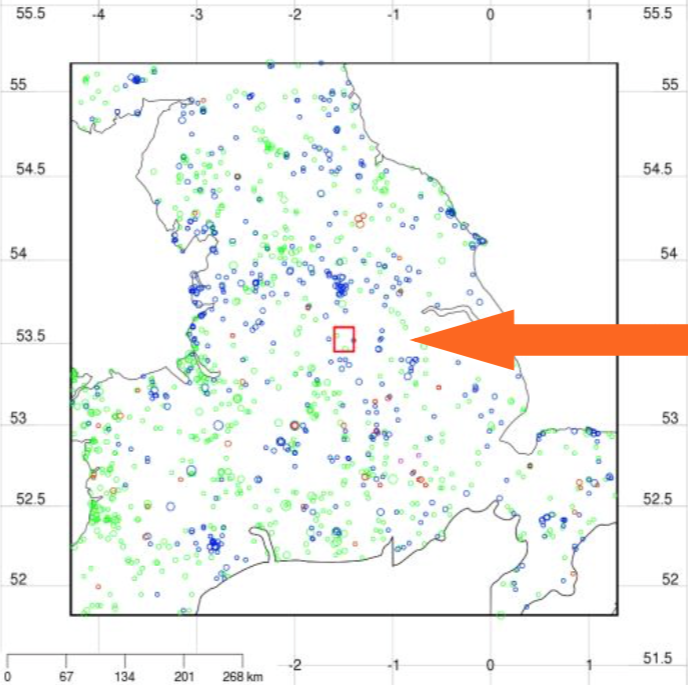
Here we explain how to interpret each component of the LEFT report, with reference to an example analysis run in the UK.
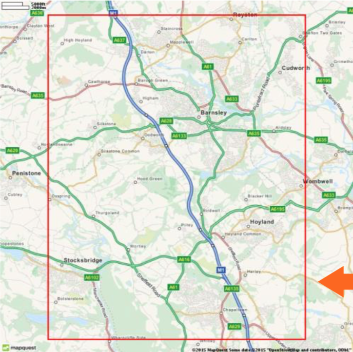
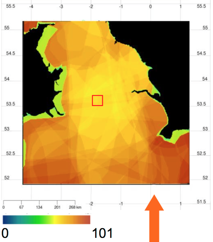
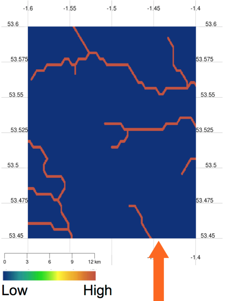
To place the analysis in a societal context, a topographic map using data from Open Street Map is included, showing roads, settlements and coastline, annotated with place names.
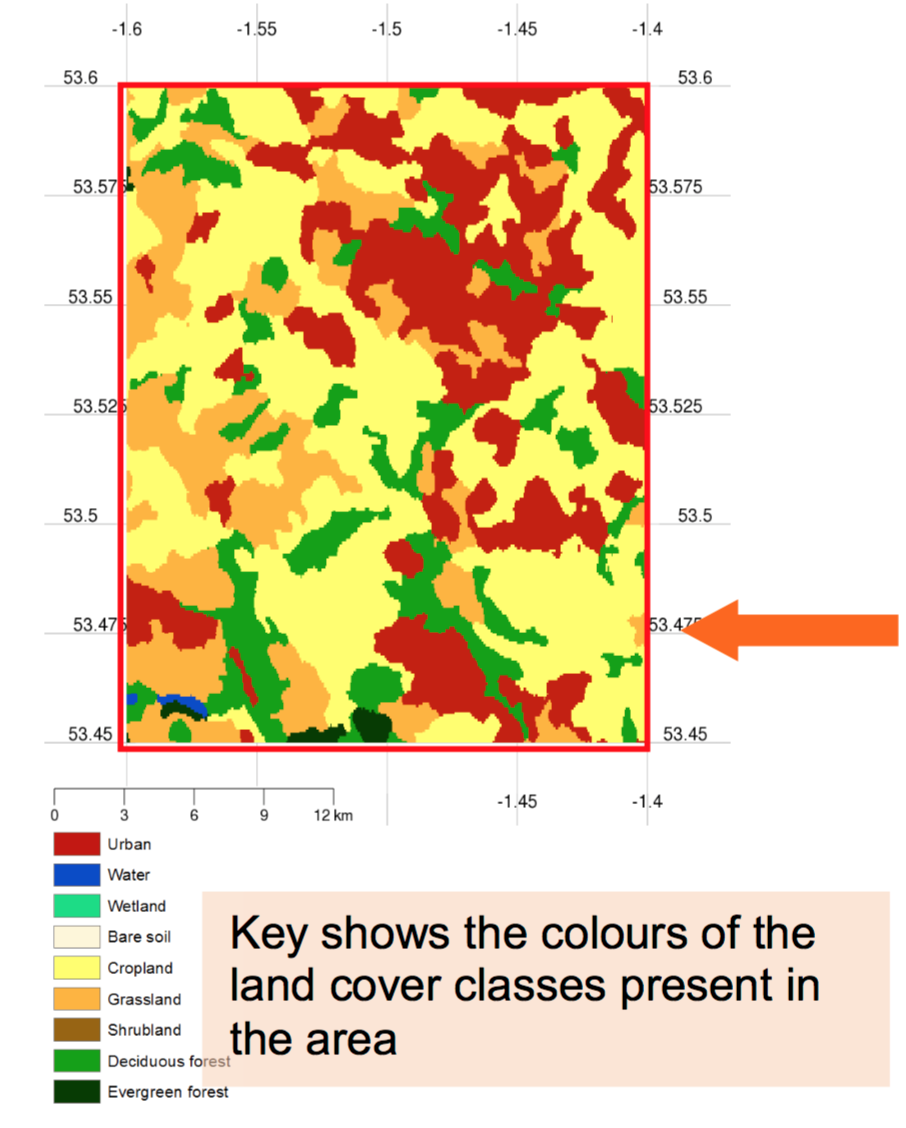
A globally consistent land cover classification using recent 30m resolution satellite data to identify the distribution of major land cover classes in the area of interest.
WWF has defined a global set of terrestrial ecoregions – areas of broadly similar climate and with similar plant and vertebrate species.
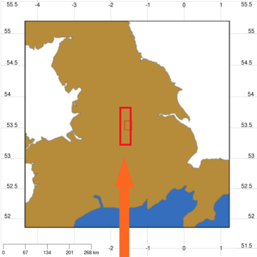
Shows which ecoregions are present in the area of interest and surrounding area – placing the analysis in the wider ecological context
Map extent is the area of interest plus a fixed 300km on all sides.
Observations of plants, amphibians, reptiles, birds and mammals are retrieved from the GBIF database and used to model patterns of biodiversity.
Map shows locations of all observations within a fixed 300km of the area of interest within ecoregions which occur in the area of interest

Table show how many individual records are available for each group within 300km of the area of interest, eg 104 bird observations, and how many different species this represents, eg records of 25 different bird species.
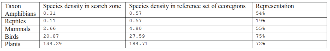
It is important to check whether the available species records are adequate to represent the biodiversity of the area of interest before further analyses are done. The number of different species for which observations are available within 300km of the area of interest is compared to the number of species which live in each of the ecoregion within 300km of the area of interest. The species density metric takes account of species-area relationships, to estimate for how representative the available records are for each taxonomic group. The units of species density are species per scaled unit area.
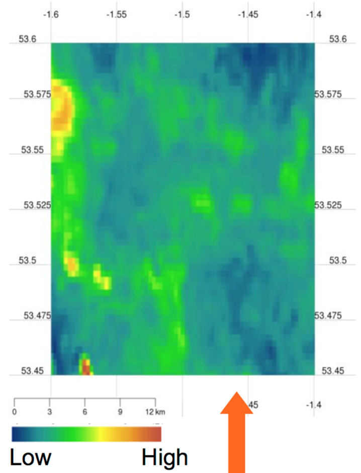
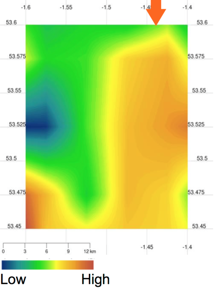
The species records from GBIF and maps of environmental variables such as temperature and rainfall are used to make a statistical model of beta-diversity. Beta-diversity is the rate of turnover in the set of species present as you move across the landscape. Important areas of high beta-diversity have strong gradients in environmental variables -very different ecological communities (sets of species) are found when moving a short distance across the landscape. Areas of low beta-diversity are more homogenous in terms of environmental variables and the ecological communities present.
The IUCN maintains the Global Redlist, a database of species which have been evaluated against criteria for their risk of extinction. We have used the Redlist to identify critically endangered, endangered, vulnerable and near threatened plant and vertebrate species. We have used all location records of these species from their worldwide distribution from GBIF and maps of environmental variables to model the geographic distributions of all species for which enough records are available. The vulnerability layer in LEFT shows how many different threatened species are potentially present across the landscape. The most important areas are those which provide a habitat for the greatest numbers of threatened species.
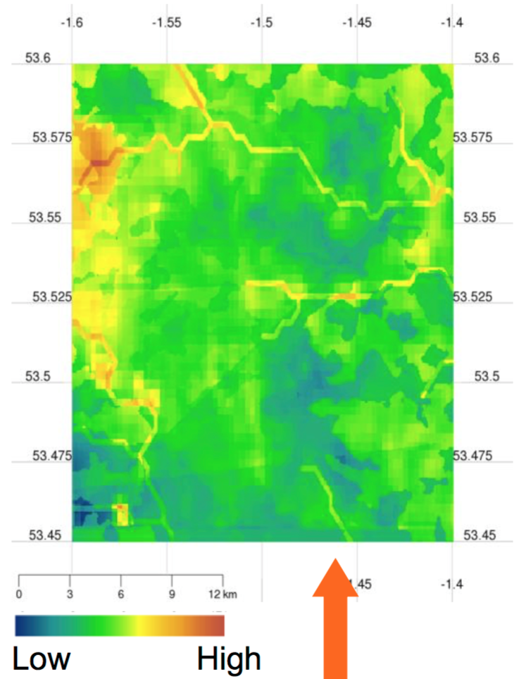
The land cover map is used to calculate the area of each contiguous patch of the same land cover class e.g. a patch of forest or a patch of grassland. This allows a map of habitat patch size to be produced. Low values correspond with very small patches of highly fragmented habitat. High values correspond with important large patches of unfragmented habitat.
To identify whether the area of interest is important in providing connectivity to migratory species, we have used the GROMS database of migratory species to show, at a regional scale, how many different migratory species are potentially dispersing across the area of interest. Important areas are those which are potentially traversed by a large number of different migratory species.
Wetlands support dispersal by many species. We have used the land cover classification as well as the Hydrosheds dataset on stream channels to identify the important parts of the area of interest which are close to wetlands and streams.
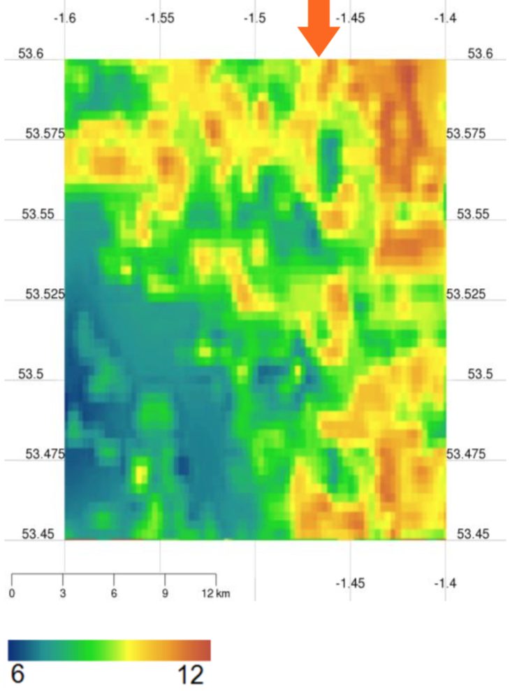
We have used a long time-series of satellite observations of vegetation greenness as well as a time-series of satellite observations of air temperature, water availability and light availability to characterise the resilience of vegetation to variation in these climate variables.
High values of resilience indicate important areas where vegetation has maintained greenness despite variation in climate variables. Low values of resilience indicate areas where vegetation greenness has changed when climate anomalies have occurred.
The LEFT report provides information on the relative importance in the area of interest of five complementary components:
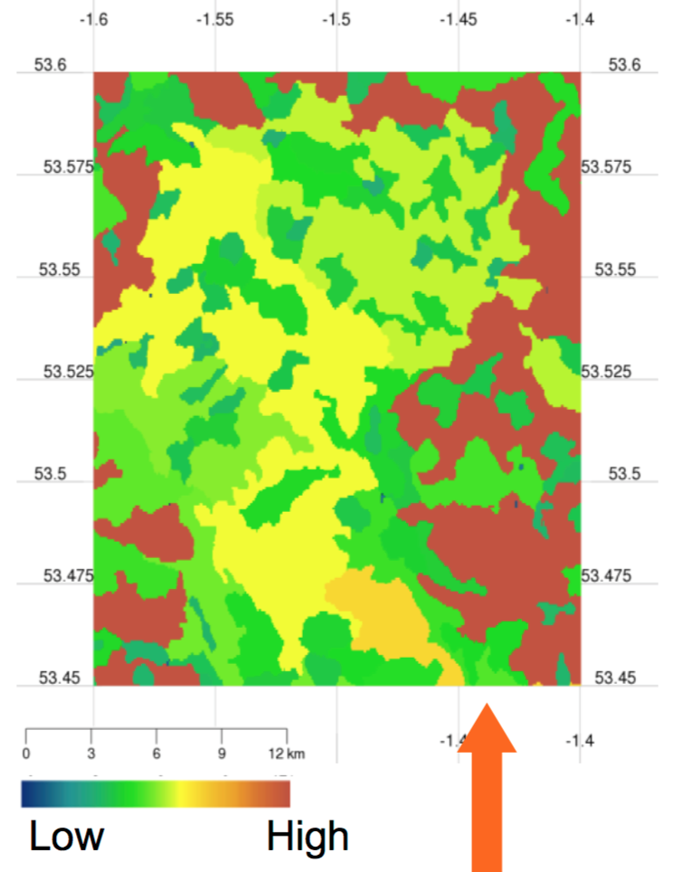
A summary ecological value (SEV) map is produced by standardising each component so that each contributes equally and then aggregating them into a single map. This map identifies areas of high SEV which are consistently important across many different components of ecological value.
The LEFT report shows which parts within the area of interest are most ecologically important.
The management information component of LEFT attempts to place these results into a broader context by showing how important the area of interest is with respect to each component of ecological value compared with a wider reference region - the ecoregions within 300km of the area of interest.
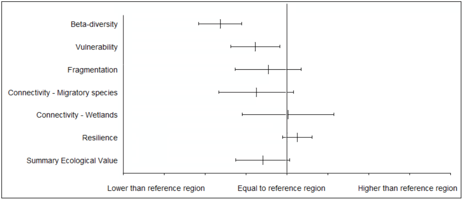
The management information graph shows that, for example, the beta diversity of this area of interest is lower than the average for comparison ecoregions, and that the area of interest is more resilient than the average for the comparison ecoregions.
This information can help judge the significance of each layer. For example if the management graph were to show that an area of interest is exceptionally important in terms of numbers of vulnerable species compared to the ecoregion, then the parts of the landscape identified in the vulnerability map as providing habitat for large numbers of threatened species become even more important when considered in a regional context.
Conversely, if this graph shows that an area of interest is regionally unimportant with respect to a component of ecological value, even the locations in the area of interest with the highest values for that component may not be very important in the regional context.